and it is deadly simple

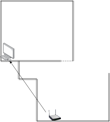
So, here is the problem. Although my apartment is just a small one and the distance between the Wifi router and my PC is also not far, they are separated by some wall layers.

just a blog post for summarizing my algorithm learning course.

1. Line segment intersection problem

Given N horizontal and vertical line segments, find all the points where they intersect, given that all x- and y-coordinates (of every endpoint) are distinct

Quadratic algorithm: check every pair of segments for intersection - O(N²).

2. Sweep-line idea

A vertical segment can only ever intersect a horizontal one, so the search really comes down to: for every vertical segment, which horizontal segments cross it?

Instead of comparing every pair, sweep an imaginary vertical line across the plane from left to right. The x-coordinate of every endpoint becomes an event, and events are processed in x-order:

• h-segment, left endpoint: insert its y-coordinate into a BST - the segment is now “active” (it currently crosses the sweep line).
• h-segment, right endpoint: remove its y-coordinate from the BST - the segment is no longer active.
• v-segment: since a vertical segment lives entirely at one x-coordinate, do a 1d range search in the BST for the segment’s [y_lo, y_hi] interval - every active h-segment whose y-coordinate falls in that range crosses the vertical segment right here.

In other words, the BST always holds the y-coordinates of the h-segments the sweep line is currently passing through, and a v-segment turns into exactly the 1d range search from the previous post.

3. Worked example

Take four h-segments and one v-segment (all x-coordinates distinct, as the nondegeneracy assumption requires):

• 0: y = 0, x from 0 to 11
• 1: y = 1, x from 1 to 8
• 2: y = 2, x from 2 to 4
• 3: y = 3, x from 3 to 9
• 4 (vertical): x = 6, y from 0.5 to 2.5

Processing events left to right:

By the time the sweep line reaches the v-segment at x = 6, segment 2 has already been deleted (its right endpoint was at x = 4), so the BST only holds {0, 1, 3}:

The range search for [0.5, 2.5] only matches 1 (green): 0 is below the range and 3 is above it, so segment 4 intersects only segment 1, at the point (6, 1).

4. Sweep-line characteristics

The sweep-line algorithm takes time proportional to N log N + R to find all R intersections among N orthogonal line segments.

The sweep line reduces 2d orthogonal line segment intersection search to 1d range search - the same O(log N) insert/delete and O(R + log N) range search from a balanced BST carry straight over, just applied once per event instead of once overall.

just a blog post for summarising my algorithm learning course.

1. What is 1D Range Search?

Think of it as the extension of Symbol Table

• Range search: find all keys between k1 and k2.
• Range count: the number of keys between k1 and k2.

Application: Database queries.

Geometric: think of the keys as points on a line - range search/count then just means finding/counting the points that fall inside a given 1d interval. This shows up directly in database queries (WHERE k1 <= key AND key <= k2).

Here’s a small ordered symbol table built by inserting J C T A M F R one at a time, followed by a count and a search for the range D to N:

2. List/Array implementations

Before reaching for a BST, consider the two obvious data structures:

• Unordered list: insert is O(1) (just append), but a range search/count has to scan every key, so it’s O(N).
• Ordered array: insert has to shift elements to keep the array sorted, so it’s O(N), but a range search/count can binary search for the position of k1 and k2 and then just walk (or count) the keys in between.

N is the number of keys in the table, R is the number of keys that match the query. Neither elementary structure hits the goal row - a balanced BST does, as the next two sections show.

3. Range count in a BST

Reuse the rank(key) operation from an ordinary BST (the number of keys strictly less than key) to answer a range count in two rank queries:

public int size(Key lo, Key hi)
{
    if (contains(hi)) return rank(hi) - rank(lo) + 1;
    else              return rank(hi) - rank(lo);
}

For example, in this BST the rank of each key is shown in parentheses:

Running time: proportional to log N.

rank() walks a single search path, so size(lo, hi) only touches the nodes on the search path to lo plus the nodes on the search path to hi - both O(log N) in a balanced BST.

4. Range search in a BST

Range count only needs two ranks, but range search has to actually collect every matching key. The recursive strategy prunes whole subtrees that can’t contain a match:

• Recursively search the left subtree, but only if it could contain a key >= lo.
• Check whether the key at the current node falls in [lo, hi]; if so, add it to the result.
• Recursively search the right subtree, but only if it could contain a key <= hi.

private void range(Node x, Key lo, Key hi, Queue<Key> result)
{
    if (x == null) return;

    int cmplo = lo.compareTo(x.key);
    int cmphi = hi.compareTo(x.key);

    if (cmplo < 0)              range(x.left, lo, hi, result);
    if (cmplo <= 0 && cmphi >= 0) result.enqueue(x.key);
    if (cmphi > 0)               range(x.right, lo, hi, result);
}

Searching the same tree for the range [D..N]:

• Green nodes (J F M) fall inside [D..N] and are added to the result.
• Red nodes (C T R) are compared against but don’t match: C < D so its left subtree (A, greyed out) is skipped entirely, and T > N so its right subtree is skipped too.
• Grey nodes are never even visited - that’s the pruning at work.

Running time: proportional to R + log N.

The nodes examined are the search path to lo, plus the search path to hi, plus the R matches themselves - each of those three pieces is bounded, so the total stays close to R + log N even though the recursion visits the whole tree in the worst case (e.g. a query that matches every key).

5. Summary

Backed by a balanced BST (a red-black BST or a B-tree), 1d range search hits the goal row from the table above: O(log N) insert, O(log N) range count, and O(R + log N) range search - all without giving up any of the ordered symbol table’s other operations.

just a blog post for summarising my algorithm learning course.

Left-leaning Red-black BST

1. From main memory to disk

2-3 search trees and red-black BSTs both assume the whole structure lives in memory, where every comparison costs roughly the same. Once the symbol table is too big for memory - a database, a file system - a different cost dominates: reading a chunk of data off disk.

File system model:

• A page is a contiguous block of data (e.g. a file, or a 4,096-byte chunk).
• A probe is the first access to a page (e.g. transferring it from disk into memory).
• A probe is much slower than comparing keys already in memory.
• Cost model: number of probes.
• Goal: access data using the minimum number of probes.

2. B-trees

B-tree (Bayer-McCreight, 1972). Generalize a 2-3 tree by allowing up to M - 1 key-link pairs per node - choose M as large as possible so that M links fit in one page (e.g. M = 1024).

• At least 2 key-link pairs at the root.
• At least M / 2 key-link pairs in every other (internal) node.
• At most M - 1 key-link pairs in any node.
• External nodes (the bottom level) hold the actual client keys.
• Internal nodes hold copies of keys, purely to guide the search - each key in an internal node is a copy of the smallest key in the subtree below it.
• A sentinel key *, smaller than every possible client key, is kept in the leftmost slot of the leftmost node on every level, so that node still has one more link than it has “real” keys.

Here’s a B-tree of order M = 6 (so every node holds between 3 and 5 key-link pairs, except the root):

The root is a 2-node (2 key-link pairs). *, 20, 35 and 50, 65, 75 are internal 3-nodes. 50, 52, 55, 58, 60 is a full external 5-node (M - 1 = 5 keys), and every other leaf is a 3- or 4-node. Notice 20, 35, 50, 65 and 75 each appear twice: once as a guide key in an internal node, and once as the smallest client key of the leaf it points to.

3. Search in a B-tree

• Start at the root.
• Find the interval containing the search key and follow the corresponding link.
• Repeat until the search terminates in an external node.

Example: searching for 68 follows the right link at the root (68 >= 50), then the middle link at 50, 65, 75 (68 is between 65 and 75), landing in the external node 65, 68, 70:

Most other read-only operations (floor, ceiling, iteration, …) work the same way - always following the single interval that contains the key.

4. Insertion in a B-tree

• Search for the new key, as above; this always terminates in an external node.
• Insert the new key into that external node, in order.
• If the node now has M key-link pairs (overflow), split it into two half-full nodes and push a copy of the new node’s smallest key up into the parent - which may itself overflow and split, and so on, possibly all the way up to the root.
• If the root splits, create a brand-new root above it with one key and two links. This is the only way a B-tree grows in height, and it does so uniformly across every leaf - the tree stays perfectly balanced.

Worked example, starting from a small order-6 B-tree whose root is already a full 5-node:

Inserting 100 (the new smallest key) lands in the leftmost leaf, which now has 6 key-link pairs - one too many:

That leaf splits into *, 100, 103 and 105, 108, 112, pushing a copy of 105 up into the root - which now overflows too (6 key-link pairs):

The root splits too, into *, 105, 130 and 160, 190, 220, and a brand-new root *, 160 is created above them - the tree just grew by one level, uniformly across every leaf:

5. Balance in a B-tree

Proposition: a search or an insertion in a B-tree of order M with N keys requires between log_(M-1) N and log_(M/2) N probes.

• Every internal node (besides the root) has between M / 2 and M - 1 links, which squeezes the height between those two logarithms.
• In practice, the number of probes is at most 4 or 5 even for huge tables, because M is chosen large enough that a handful of levels covers billions of keys.
• Optimization: always keep the root page in memory - that’s one guaranteed probe saved on every single search or insert.

Splitting always divides an overflowing node into two halves, so right after a split each half is about half full; as more keys are inserted into the surrounding leaves those pages gradually fill back up until they overflow and split again:

6. B-trees in the wild

B-tree variants - B+ tree, B* tree, B# tree, … - are widely used for file systems and databases, where minimizing the number of page reads matters far more than the number of comparisons:

• Windows: NTFS.
• Mac: HFS, HFS+.
• Linux: ReiserFS, XFS, Ext3FS, JFS.
• Databases: Oracle, DB2, INGRES, SQL Server, PostgreSQL.

Compare that to the red-black BSTs from the previous post, which shine as in-memory symbol tables - both are ultimately descendants of the same idea, a 2-3 tree, just tuned for very different costs: comparisons in memory vs. probes on disk.

just a blog post for summarising my algorithm learning course.

Previous post: 2-3 search trees

1. From 2-3 trees to red-black BSTs

• 2-3 search trees give guaranteed log N search/insert, but implementing 3-nodes directly is annoying: multiple node types, multiple compares to move down, and a bunch of cases for splitting.
• Left-leaning red-black BST (LLRB): represent a 2-3 tree as an ordinary BST, and use “internal” left-leaning links as glue to hold the two keys of a 3-node together.

• A 3-node p,q (p < q) has three children - for keys smaller than p, between p and q, and larger than q:

  graph TD PQ(("p, q")) --> L1("< p") PQ --> L2("p..q") PQ --> L3("> q")

• It’s encoded as two 2-nodes: q becomes a plain black node, and p hangs off its left as a red child. The three original children still hang in the same relative positions - q keeps the > q child, and p takes the other two. The red link is just bookkeeping - it says “these two nodes are really one 3-node”:

  graph TD Q((q)) --> P((p)) Q --> R3("> q") P --> R1("< p") P --> R2("p..q") linkStyle 0 stroke:#c00,stroke-width:3px

• Here’s that same idea inside an actual tree. The 2-3 tree below has H,L as one of its 3-nodes:

  graph TD R((R)) --> HL(("H, L")) R --> X((X)) HL --> A((A)) HL --> J((J)) HL --> M((M))

• …and its red-black equivalent, where L stays a plain black node and H hangs off it as a red left child:

  graph TD R((R)) --> L((L)) R --> X((X)) L --> H((H)) L --> M((M)) H --> A((A)) H --> J((J)) linkStyle 2 stroke:#c00,stroke-width:3px

A red-black BST is a BST whose links are colored red or black, such that:

• No node has two red links connected to it.
• Every path from the root to a null link has the same number of black links (“perfect black balance”).
• Red links lean left.

Every 2-3 tree corresponds to exactly one LLRB tree: 2-nodes stay as they are, and each 3-node becomes a black node with a red left child. Take the 2-3 tree from the previous post:

Its corresponding red-black BST looks like this (red links drawn in red):

Each 3-node from the 2-3 tree (F,N, B,D and Y,Z) turned into a black node with a red left child (N←F, D←B, Z←Y); every 2-node stayed a plain black node.

2. Search

Search is exactly the same as in an elementary BST - the colors are simply ignored, it just happens to run faster because the tree is better balanced.

Example: searching for K walks T -> N -> F -> K, crossing the red link between N and F along the way:

Most other read-only operations (floor, ceiling, selection, iteration, …) are also identical to a plain BST.

public string Get(int key)
{
    Node node = root;
    while (node != null)
    {
        int cmp = key.CompareTo(node.Key);
        if (cmp < 0) node = node.Left;
        else if (cmp > 0) node = node.Right;
        else return node.Value;
    }
    return null;
}

3. Node representation

Since every node is pointed to by exactly one link (from its parent), the color can be stored on the node itself, as the color of the link coming down from its parent:

• Each node stores its key/value, its two children, and a boolean color field.
• color records whether the link from the parent to this node is red or black.
• Null links are considered black.

private const bool Red = true;
private const bool Black = false;

private class Node
{
    public int Key;
    public string Value;
    public Node Left;
    public Node Right;
    public bool Color; // color of the link from the parent to this node

    public Node(int key, string value, bool color)
    {
        Key = key;
        Value = value;
        Color = color;
    }
}

private static bool IsRed(Node node)
{
    if (node == null) return false; // null links are black
    return node.Color == Red;
}

4. Elementary operations

Every red-black BST operation is built from three tiny local operations. Each one preserves symmetric order and perfect black balance.

4.1 Rotations

Left rotation - orient a (temporarily) right-leaning red link to lean left:

becomes

Right rotation is just the mirror image - it orients a left-leaning red link to (temporarily) lean right, turning the “after” picture above back into the “before” one. Both rotations keep the subtree’s in-order sequence unchanged; only the shape and the position of the red link change.

private Node RotateLeft(Node h)
{
    Node x = h.Right;
    h.Right = x.Left;
    x.Left = h;
    x.Color = h.Color;
    h.Color = Red;
    return x;
}

private Node RotateRight(Node h)
{
    Node x = h.Left;
    h.Left = x.Right;
    x.Right = h;
    x.Color = h.Color;
    h.Color = Red;
    return x;
}

4.2 Color flip

Recolors a node and its two children to split a temporary 4-node. Before the flip, a black node has two red children:

After the flip, G and U turn black, and O itself turns red (so its own link to its parent becomes red, ready to be dealt with one level up):

private void FlipColors(Node h)
{
    h.Color = !h.Color;
    h.Left.Color = !h.Left.Color;
    h.Right.Color = !h.Right.Color;
}

5. Insertion

The strategy is always the same: do a normal BST insert, attach the new node with a red link, then walk back up the search path fixing any violations using the three operations above.

5.1 Case 1: insert into a 2-node

If the new key is smaller, it simply attaches as a red left child - already a valid 3-node, no fix-up needed. If it’s larger, it attaches as a red right child, which is not allowed to lean right, so a left rotation fixes it.

Going back to the tree above, let’s insert X, which belongs under the leaf V:

X is attached as a red right child of V - a temporary, illegal right-leaning red link. A single left rotation at V fixes it: X takes V’s place under W, with V hanging off as its red left child:

No violation reaches W, so the insertion is done in a single rotation.

5.2 Case 2: insert into a 3-node

This is where a rotation and a color flip usually happen together. Take a standalone 3-node G,O (G is O’s red left child):

Insert a key C smaller than G. It attaches as a red left child of G:

Now there are two left-leaning red links in a row (O -> G -> C), which breaks the “no two reds in a row” rule. A right rotation at O fixes the lean - G takes O’s place, with C and O as its two red children:

G now has two red children - a temporary 4-node - so a color flip splits it: C and O turn black, and G turns red to pass the split one level up (exactly like the middle key moving up into the parent in a 2-3 tree):

5.3 Putting it together

Walking back up from the newly inserted node, the same three checks are applied at every node on the search path:

• Right child red, left child black → rotate left (straighten a right-leaning link).
• Left child red and left-left grandchild red → rotate right (fix two lefts in a row).
• Both children red → flip colors (split a temporary 4-node, pass it up).

Repeating this at each level guarantees the red link either gets absorbed or keeps moving up, exactly as in a 2-3 tree insertion. If it reaches the root and the root ends up red, it’s simply repainted black - the only case where the tree grows one level taller.

All of this fits in a handful of lines on top of a standard recursive BST insert:

public void Put(int key, string value)
{
    root = Put(root, key, value);
    root.Color = Black; // root is always black
}

private Node Put(Node h, int key, string value)
{
    if (h == null) return new Node(key, value, Red); // insert at the bottom, link colored red

    int cmp = key.CompareTo(h.Key);
    if (cmp < 0) h.Left = Put(h.Left, key, value);
    else if (cmp > 0) h.Right = Put(h.Right, key, value);
    else h.Value = value;

    if (IsRed(h.Right) && !IsRed(h.Left)) h = RotateLeft(h);       // lean left
    if (IsRed(h.Left) && IsRed(h.Left.Left)) h = RotateRight(h);   // balance a 4-node
    if (IsRed(h.Left) && IsRed(h.Right)) FlipColors(h);            // split a 4-node

    return h;
}

6. Performance

• Every path from root to null link has the same number of black links, and no two red links ever appear in a row, so the height is at most 2 lg N in the worst case.
• In typical, non-adversarial use the height tends to be close to lg N.

7. Why red-black BSTs?

Because they get almost all of the 2-3 tree’s balance guarantees while being just a thin, constant-overhead layer on top of an ordinary BST (a single extra color bit per node, three local fix-up operations), red-black trees ended up as one of the most widely used balanced search trees in practice:

• Java’s java.util.TreeMap / java.util.TreeSet.
• .NET’s System.Collections.Generic.SortedDictionary<TKey, TValue> / SortedSet<T>.
• C++ STL’s map, multimap, multiset.
• The Linux kernel’s completely fair scheduler (linux/rbtree.h).

B-trees take a different route to the same goal - instead of 2 or 3 keys per node, they allow up to M - 1, which is a much better fit for data that lives on disk (databases, file systems) where minimizing the number of page reads matters more than the number of comparisons. See my next post

Nothing special here. It’s just a blog post for summarising my algorithm learning course.

1. Compare to BST

• Symbol Tables and Binary Search Trees summary

2. What is a 2-3 tree?

A 2-3 tree is a tree that guarantees log N search/insert/delete by allowing a node to hold 1 or 2 keys instead of just 1.

• 2-node: one key, two children (same as a regular BST node).
• 3-node: two keys, three children (smaller, in the middle and larger).
• Symmetric order: an in-order traversal still yields the keys in ascending order.
• Perfect balance: every path from the root to a null link has the same length.

F,N, B,D and Y,Z are 3-nodes (2 keys, drawn in red above); the rest are 2-nodes. Following the F,N node: the left link leads to keys smaller than F, the middle link to keys between F and N, and the right link to keys larger than N - same idea as a 3-way BST node.

3. Search

• Compare the search key against the keys in the node.
• Find the interval containing the search key.
• Follow the associated link, recursively.

Example: searching for K walks T -> F,N -> K:

4. Insertion

Insertion always happens at the bottom (a leaf). Inserting into a 3-node at the bottom works like this:

• Add the new key to the 3-node, creating a temporary 4-node.
• Move the middle key of the 4-node up into the parent.
• Repeat up the tree, as necessary, since pushing a key into the parent can turn the parent into a temporary 4-node too.
• If the split reaches the root and the root itself is a 4-node, split it into three 2-nodes - this is the only way the tree grows taller.

4.1 Splitting a 4-node

Splitting a temporary 4-node is a local transformation - a constant number of nodes/links change, regardless of the size of the tree. Before splitting, p,t has a temporary 4-node child q,r,s:

After splitting, q,r,s becomes three separate 2-nodes and the middle key r moves up into the parent:

The middle key r moves up one level into the parent (as p, r, t), while q and s become new 2-nodes hanging below it.

4.2 Worked example

Starting from the tree above, let’s insert C. First, walk down the tree the same way Search does, to find the leaf where C belongs: T -> F,N -> B,D:

C lands in the B,D leaf. Since B < C < D, it slots in between them, temporarily turning the leaf into a 4-node B,C,D:

The leaf splits: B and D become plain 2-nodes, and the middle key C moves up into the parent F,N. Since F,N is already a 3-node, absorbing C turns it into a temporary 4-node C,F,N:

The split repeats one level up: C,F,N splits into 2-nodes C and N, and the middle key F moves up into the root. The root T was only a 2-node, so it simply absorbs F and becomes the 3-node F,T - no further splitting needed, and the tree’s height stays the same:

The final tree, still perfectly balanced and in symmetric order:

5. Global properties

Since every transformation is local and preserves symmetric order + perfect balance, the whole tree stays sorted and balanced no matter where the temporary 4-node appears:

• Root is a 4-node - split into three 2-nodes; this is the only case where the tree height grows. Before splitting, the root is a temporary 4-node p,q,r:

  graph TD PQR(("p, q, r"))

  After splitting, the root becomes the 2-node q, with p and r as its two children:

  graph TD Q2((q)) --> P2((p)) Q2 --> R2((r))
• Parent is a 2-node - the 4-node is either the parent’s left or right child; the parent simply absorbs the middle key and becomes a 3-node. No further splitting is needed.
• Parent is a 3-node - the 4-node is the parent’s left, middle, or right child; the parent absorbs the middle key and itself becomes a temporary 4-node, so the split repeats one level up.

Because each split only ever moves one key up per level, an insertion costs at most O(tree height) splits.

6. Performance

• Worst case height: lg N - a tree made entirely of 2-nodes (behaves like a plain BST).
• Best case height: log₃ N ≈ 0.631 lg N - a tree made entirely of 3-nodes.
• Between 12 and 20 for a million nodes.
• Between 18 and 30 for a billion nodes.
• Guaranteed logarithmic performance for both search and insert, no matter the insertion order.

7. Why not implement it directly?

Direct implementation is complicated because:

• Maintaining multiple node types (2-node vs 3-node) is cumbersome.
• Multiple compares are needed just to move down the tree.
• You need to move back up the tree to split 4-nodes.
• There’s a large number of cases for splitting (see the six cases above).

In practice, 2-3 trees are usually implemented indirectly through left-leaning red-black BSTs, which encode a 3-node as two 2-nodes joined by a left-leaning red link - same performance guarantees, much simpler code. See next post

Left-leaning Red-black BST

Nothing special here. It’s just a blog post for summarising my algorithm learning course. Although this was already taught in the University, it’s still god to summarize here

1. Symbol Tables

Key-value pair abstraction.

• Insert a value with specified key.
• Given a key, search for the corresponding value.

Example

Symbol Table APIs

Symbol Tables act as an associative array, associate one value with each key.

public class ST<Key, Value> {
    void put(Key key, Value, val);
    Value get(Key key);
    void delete(Key key);
    boolean contains(Key key);
    boolean isEmpty();
    int size();
    Iterable<Key> keys();
}

At the time of this writing, I have been working at Agency Revolution (AR) for more than 2 years, on a product focusing mostly on automation email marketing for the Insurance Agencies. I have been working on this product since it was in beta, when it could only serve only a few clients, send thousands of emails each month and handle very little amount of integration data without downtime until it can deliver millions of emails each month, store and react to terabytes of data flow every day. The dev team has been working very hard and suffering a lot of problem to cope with the increasing number of customers that the sale team brought to us. Here the summary of some techniques and strategies that we have applied in order to deliver a better user experience.

The problem of On-demand computing

By On-demand, I mean the action of computing the required data only when it is needed.

One of the core value of our system is to deliver the right messages to the right people at the right time. Our product allows users to set up automated emails, which will be sent at a suitable time in the future. The emails are customised to each specific recipient based on their newest data at the time they receive the email, for example the current customer status, whether that customer is an active or lost customer at that time, how many policies he/she has or the total value that customer has spent until that time.

Part 1 here Some Optimizations in RethinkDB - Part 1

Yes, it’s RethinkDB, a discontinued product. Again, read my introduction in the previous post. It’s not only about RethinkDB but it also the basic idea for many other database systems. This post introduces other techniques that I and the team have applied at AR to maximize the workload that RethinkDB can handle but most of them can be applied for other database systems as well.

Increase the Memory with NVME SSD

Well, sound like a very straight forward solution, huh? More memory, better performance, sound quite obvious! Yes, the key thing is how to increase the memory without significant cost. The answer is to setup swap as the temporary space for storing RethinkDB cached data. RethinkDB, as well as other database systems, caches the query result data into memory so that it can be re-used next time the same query executes again. The problem is that swap is much slower than RAM, because we rely on the disk to store the data. However, since we are running on Google Cloud and Google Cloud offers the Local-SSDs solution, we have been exploiting this to place our swap data. Here is the Local-SSDs definition, according to Google

Local SSDs are physically attached to the server that hosts your virtual machine instance. Local SSDs have higher throughput and lower latency than standard persistent disks or SSD persistent disks. The data that you store on a local SSD persists only until the instance is stopped or deleted.

Feature Toggle is a very popular technique that enables you to test the new feature on real production environment before releasing it to your clients. It’s also helpful when you want to enable the feature for just some beta clients or just some clients who pay for the specific features. The technique requires both backend and frontend work involved. In this post, I’m going to talk about some simple solutions that I and the team at AR have applied as well as some other useful ways that we are still discussing and may apply one day in the future.

1. Backend Data Organization

Feature Flag table

Of course, the simplest solution is to create a specific table for storing the all the feature flags in the database. The table may looks like this

{
  featureName: <string>,
  released: <bool>,
  enabledList: <array>, // enabled clients list
  disabledList: <array> // disabled clients list
}

The above mentioned data structure may be suitable for the case your system has a lot of users. You can simply add some admin user to the enabledList and test the new feature on production before releasing it to your users.

Inline User feature data

If your product is to serve business clients, you can also store the enabled feature directly to the client object itself. This can save you extra queries to the database to get the feature information. If that’s the case, your Client object might look like this

{
  clientId: <string>,
  enabledFeatured: <array>
}

Unix Permission style